English

English

Monopoly IB

Target Question:

How does a monopoly maximise profit and what are the welfare effects in IB Economics?

Full activity practice breakdown, exam practice, model answers and evaluation tools are available exclusively in the IB Economics Activity Book.

IB Economics: Monopoly - Theory, Diagrams and Welfare Analysis

Everything about monopoly you need main concepts, diagrams and required critical thinking for your IB Economics course - market power, profit maximisation, efficiency analysis, price discrimination, and welfare effects.

What Is a Monopoly?

A monopoly happens when a single firm is the sole supplier of a good or service with no close substitutes, protected from competition by significant barriers to entry. The monopolist is a price maker - unlike a firm in perfect competition, it faces the entire market demand curve and can choose its price, subject to what consumers are willing to pay.

The degree of monopoly power varies: pure monopoly (one firm, 100% market share) is rare, but significant monopoly power - the ability to sustain prices above marginal cost - is common across many industries.

IB Economics definition:

A monopoly is a market structure in which a single firm supplies the entire market, protected by barriers to entry. As the sole price maker, the monopolist maximises profit by producing where marginal cost equals marginal revenue, resulting in a price above marginal cost, supernormal profit, and a deadweight welfare loss.

Barriers to Entry: The Foundation of Monopoly

Monopoly power can only be sustained if barriers to entry prevent rivals from entering the market and competing away supernormal profits. IB Economics identifies three main types:

Natural barriers - economies of scale mean that one large firm can supply the entire market at lower average cost than multiple smaller firms. The typical examples are utilities (water, electricity distribution, railways). The high fixed costs of infrastructure create such large scale advantages that duplication by a competitor is economically irrational - this is the basis of natural monopoly.

Legal barriers - patents grant inventors a temporary legal monopoly (typically 20 years) to recoup R&D investment. Pharmaceutical companies are the most commonly examined example: a patented drug can be priced far above production cost while the patent holds. Government licences and franchises can also confer exclusive market rights.

Strategic barriers - established firms may deliberately deter entry through predatory pricing (temporarily pricing below cost to eliminate a new entrant), exclusive dealing arrangements, or control over essential inputs or distribution channels.

Brand loyalty and switching costs - while not an absolute barrier, strong brands and proprietary ecosystems (Apple's iOS, for example) raise the effective cost of switching for consumers, giving established firms persistent pricing power.

Monopoly Revenue Curves

Understanding monopoly requires clarity on revenue curves - this is where the monopoly diagram differs fundamentally from perfect competition.

In perfect competition, the demand curve facing an individual firm is perfectly elastic (horizontal) - the firm can sell any quantity at the market price. In monopoly, the firm faces the downward-sloping market demand curve - to sell more, it must lower the price on all units.

This means:

Average Revenue (AR) = the demand curve (price per unit at each quantity)
Marginal Revenue (MR) lies below the AR curve and falls twice as steeply

The main concept: MR falls below AR because selling one more unit requires reducing the price not just on the new unit but on all previous units. For a linear demand curve, MR has the same vertical intercept as AR but twice the slope.

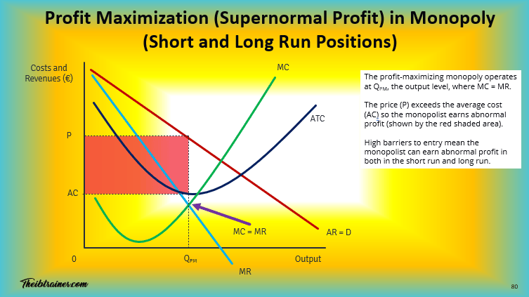
Profit Maximisation: The MC = MR Rule

A monopolist - like any firm - maximises profit by producing where Marginal Cost (MC) = Marginal Revenue (MR). This is the profit-maximising output level (Qm).

The price charged (Pm) is then read from the demand curve at Qm - the highest price consumers will pay for that quantity. Since the demand curve lies above MR, this price is always above marginal cost - the defining inefficiency of monopoly.

Supernormal (abnormal) profit - the area between price (Pm) and average total cost (ATC) at Qm, multiplied by output. In monopoly, barriers to entry prevent new firms from competing this profit away in the long run - supernormal profits can persist indefinitely.

Key diagram requirements for IB Economics:

Downward-sloping demand (AR) curve
MR curve below AR, falling twice as steeply
U-shaped ATC and MC curves
MC = MR at profit-maximising output (Qm)
Pm read vertically from Qm to the demand curve
Supernormal profit rectangle (shaded)
Deadweight loss triangles (shaded)

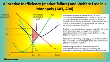
Welfare Analysis: The Cost of Monopoly

The welfare comparison between monopoly and perfect competition is one of the most important diagrams in IB Economics.

In perfect competition, the long-run equilibrium is where P = MC = minimum ATC - achieving both allocative efficiency (P = MC) and productive efficiency (production at minimum ATC). No supernormal profit persists.

In monopoly:

Allocative inefficiency - the monopolist produces at P > MC. This means consumers value additional units more than they cost to produce, but production is withheld to maintain the higher price. Resources are misallocated: too little of the good is produced relative to the social optimum.

Productive inefficiency - without competitive pressure, the monopolist need not produce at minimum average cost. X-inefficiency (production above minimum cost due to absence of competitive discipline) may also arise.

Deadweight welfare loss - the triangular area between the competitive output and the monopoly output, bounded above by the demand curve and below by the MC curve. This represents the welfare gain that would be achieved if output expanded from Qm to the competitive level - it is the efficiency cost of monopoly.

Income redistribution - monopoly transfers consumer surplus to the producer in the form of supernormal profit. This is a distributional concern separate from the efficiency loss.

Price Discrimination Under Monopoly

Price discrimination is only possible for firms with market power - it requires the ability to set prices above marginal cost and to identify and separate consumer groups. Monopolists are therefore the primary context in which price discrimination is analysed.

Third-degree price discrimination is the most commonly examined in IB Economics: charging different prices to different identifiable consumer groups based on their price elasticity of demand. Students pay less for cinema tickets than adults; peak-time train fares exceed off-peak fares; pharmaceutical companies charge different prices in different countries for identical drugs.

Conditions required: market power (the firm must be a price maker); ability to identify and separate groups with different elasticities; prevention of resale between groups.

Welfare evaluation of price discrimination: it increases the monopolist's profit by extracting more consumer surplus. Its effect on total welfare is ambiguous - output may increase compared to simple monopoly (reducing deadweight loss) or decrease. Students and lower-income consumers may gain access at lower prices, while higher-income consumers pay more. This makes price discrimination a genuine evaluation challenge rather than simply good or bad.

The Dynamic Efficiency Argument

The most important evaluative counter-argument to the standard welfare case against monopoly is dynamic efficiency. Monopoly supernormal profits provide both the funds and the incentive for research and development investment.

Schumpeter's creative destruction - Schumpeter argued that the prospect of temporary monopoly profits is the primary incentive for innovation. Firms invest in R&D because success brings monopoly pricing power. Prohibiting monopoly profits or breaking up dominant firms could reduce innovation incentives and harm long-run economic welfare more than the static deadweight loss.

This argument is strongest for:

Patent-protected pharmaceutical innovation (the patent system explicitly creates temporary monopoly as an innovation incentive)
Technology industries where R&D investment is enormous and imitation is easy without IP protection

It is weakest for:

Natural monopolies in stable utility industries (innovation is not the primary concern)
Monopolies maintained by anti-competitive practices rather than superior innovation

Exam principle: the static welfare analysis (deadweight loss) makes monopoly look unambiguously harmful. The dynamic efficiency argument is the essential evaluation that prevents this from being too simple.

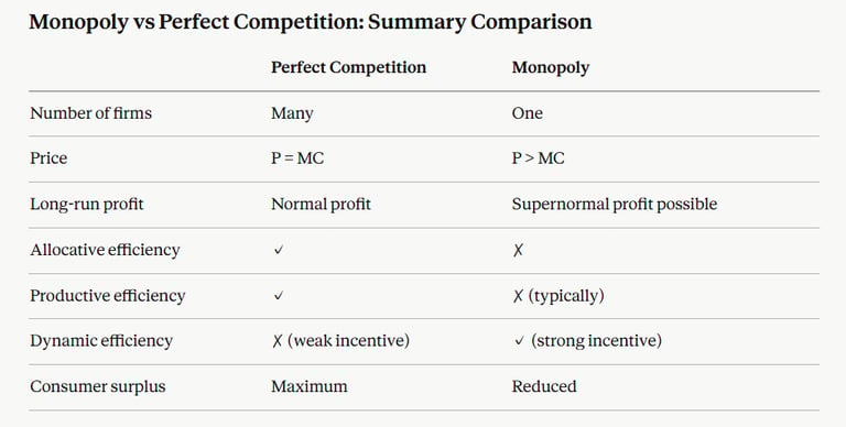
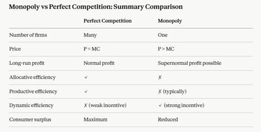
Monopoly vs Perfect Competition: Summary Comparison

Monopoly in the IB Economics Exam

Monopoly is one of the most heavily examined topics in IB Economics microeconomics:

Paper 1 - essay questions regularly ask students to draw and explain the monopoly profit-maximisation diagram, compare monopoly with perfect competition, or evaluate whether monopoly is always harmful. The 15-mark question must include the dynamic efficiency counter-argument and a supported judgement.
Paper 2 - data response questions present industry scenarios and ask students to identify monopoly characteristics, assess welfare effects, or evaluate regulation.
Paper 3 (HL) - extended questions may integrate monopoly analysis with market failure, development economics, or international trade.

Most common exam mistakes: drawing the monopoly diagram without the deadweight loss triangles; forgetting to show the supernormal profit rectangle; comparing monopoly unfavourably with perfect competition without raising dynamic efficiency; failing to distinguish allocative from productive efficiency.

IB Economics Natural Monopoly and Regulation - Full Guide →

IB Economics Market Power - Full Guide →

IB Economics Profit Revenue and Costs - Full Guide →

IB Economics Diagrams Course

Every monopoly diagram you need - profit maximisation, welfare analysis, deadweight loss, price discrimination, and the monopoly vs perfect competition comparison - fully labelled with video support.

✔ Full monopoly profit-maximisation diagram with all areas labelled
✔ Deadweight loss and consumer surplus transfer diagrams
✔ Price discrimination (all three degrees)
✔ 200+ diagrams covering the full syllabus · Both SL and HL labelled

Explore the Diagrams Course →

Frequently Asked Questions: Monopoly in IB Economics

How does a monopoly maximise profit in IB Economics? A monopolist maximises profit by producing where marginal cost (MC) equals marginal revenue (MR). At this output level (Qm), the price is read from the demand curve - always above MC since the demand curve lies above MR. The supernormal profit is the rectangle between price and average total cost at Qm. Barriers to entry prevent competitors from eroding this profit in the long run.

Why does monopoly cause allocative inefficiency? Allocative efficiency requires P = MC - resources are allocated efficiently when the price consumers pay equals the cost of producing the last unit. A monopolist sets P > MC, meaning consumers value additional units more than they cost to produce, but the monopolist restricts output to maintain the higher price. The unrealised welfare gain is represented by the deadweight loss triangles on the diagram.

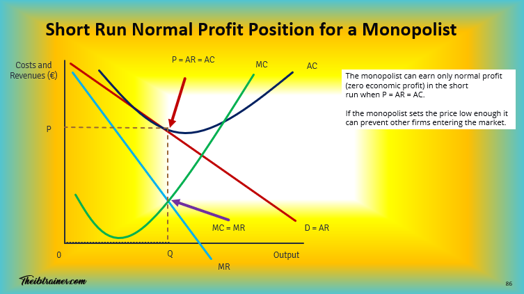
What is the difference between supernormal profit and normal profit? Normal profit is the minimum return needed to keep a firm in its current industry - it is included in economic costs. Supernormal (abnormal or economic) profit is any profit above this level. In perfect competition, supernormal profit attracts entry and is competed away in the long run. In monopoly, barriers to entry prevent this, allowing supernormal profit to persist indefinitely.

Is monopoly always harmful in IB Economics? Not necessarily - this is the essential evaluation point. The standard welfare analysis shows allocative inefficiency and deadweight loss. However, the dynamic efficiency counter-argument holds that monopoly supernormal profits fund R&D investment and incentivise innovation. Schumpeter's creative destruction suggests that monopoly positions are repeatedly challenged by new innovations, so static welfare analysis understates the long-run benefits of allowing firms to earn monopoly returns from successful innovation.

What is the relationship between the demand curve, AR, and MR in monopoly? In monopoly, the demand curve is the Average Revenue (AR) curve - it shows the price (revenue per unit) at each output level. Because lowering the price to sell one more unit reduces revenue on all previous units, Marginal Revenue (MR) falls below AR. For a linear demand curve, MR has the same vertical intercept as AR but falls twice as steeply, crossing the horizontal axis at half the output level where AR crosses it.

This hub is updated regularly to reflect current IB Economics syllabus requirements and exam developments.

Key Monopoly IB Economics Diagrams

More Information About:

IB Economics Hub Page your IB Economics daily guide

IB Economics Module 2 Microeconomics Hub Page access Monopoly here as well as the rest of the module 2

IB Economics Diagrams Page Check Unit 13 for All Market Power, Monopoly and Natural Monopoly diagrams with explanations

IB Economics Market Power Hub Page All your Monopoly, Natural Monopoly and Market Power theory in one place

IB Economics Perfect Competition Page explore the differences between Monopoly and Perfect competition here

IB Economics Activity book Page Module 2 Microeconomics Unit 2.16 for Monopoly & Natural Monopoly exam practice, activities, model answers and IB Economics Marking schemes

IB Economics Monopoly Hub Page explore Monopoly from a different angle

Revenue, Costs and Profit Page - abnormal profit in the long run links directly to monopoly; You need to go through this content to fully understand the profit analysis done for monopoly.

Market Failure Hub page - monopoly power causes allocative inefficiency; this is one of the biggest real-world sources of market failure

Government Intervention Hub page - price regulation, nationalisation, and Ofwat/Ofgem all connect directly to government intervention in markets

IB economics Calculations Book make sure you check unit 11 for Monopoly and Natural Monopoly calculations exercises, IB model answers, and IB marking schemes

Read Next: IB Economics Inequality Hub Page